We have seen how to apply ideas from physics to finance in several different sorts of ways, from introducing simple ideas like 'trade space' and a focus on empirically measurable values, to robust statistical models like the log-normal model of prices, and the Black-Scholes model of options. These tools are powerful when successful. But the techniques we have developed are also powerful in allowing us to analyse when our models fail, and explore new ways forward beyond classical finance. We are now going to turn to the latter.
Beyond Black-Scholes
In the last lecture, we discussed the Black-Scholes technique for pricing options. It is an incredibly simple technique, which works whenever a few assumptions are met: that there is no arbitrage in the market; that we can measure a risk-free interest rate; and that the price of the underlying stock is distributed on a random walk model.
The incredibly small number of assumptions needed for Black-Scholes option pricing to work means there are only a few substantial ways that Black-Scholes pricing can fail. By thinking about each of them, we can gain insight into how to improve the model in such cases.
| What fails | Why | Example |
|---|---|---|
| No Arbitrage | Arbitrage in a market might entail that the option price cannot be presumed to match its price in a risk-free portfolio. | LTCM bond arbitrage |
| Risk-free interest rate | Might have been incorrectly measured or might change, for example if we identify it with the interest rate of a bond that is higher risk than expected. | 1998 Russian default |
| Random walk | A failure of the random walk hypothesis may lead to an incorrect distribution of prices of the underlying stock, and thus an incorrect use of the variance in the Black-Scholes equation. | Volatility smile, Levy walks |
There are of course a couple of other approximations made, for example by ignoring transaction costs. But these idealisations are easily removed. The three possible failures above, in contrast, are quite substantial, and indeed have all occurred during times when there was a historic market disaster. Let's look at each of them in detail.
Arbitrage trading
John Meriwether became a star investor in the 1980's and 1990's by pioneering new methods of profiting from arbitrage while working at the Salomon Brothers investment bank. His basic method was simple: seek out differences in prices, then buy at the low price and sell at the high, thus ensuring a guaranteed profit.
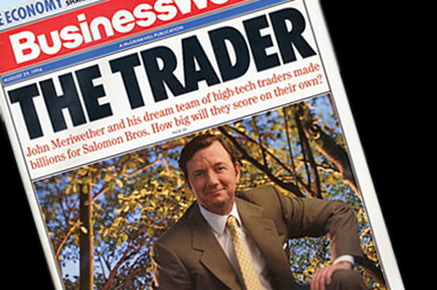
For example, deregulation Japan led to new sorts of options becoming available in the 1980s, with prices that were different from those suggested by the new option-pricing models like Black-Scholes in the United States. Once you figured this out, it was often briefly possible for you to buy at the low price and sell at the high. Meriwether reported in an interview with Donald MacKenzie that they made almost $1 billion in two years through tricks of this kind.
There is a Janus-faced feature of this kind of trade. On the one hand, it embraces the existence arbitrage, albeit sometimes briefly. On the hand, it presumes that some options will be priced using the Black-Scholes formula, which is only justified if there is no arbitrage. The logic of such a situation is delicate at best.

Nevertheless, Meriwether's success soon led him to strike out on his own, founding Long Term Capital Management (LTCM), which became a star hedge fund in the 1990s through similar techniques. Meriwether recruited Myron Scholes and Robert Merton (of Black-Scholes-Merton theory fame) for its board of directors, and soon raised over a billion dollars from investors, including the Italian government. All the way up through the end of 1997, LTCM was turning an enormous profit on their particular specialty in bond arbitrage. All the while, they profited from regular use of the Black-Scholes formula, in spite of the fact that their profits arose out of a feature that made the use of this formula illegitimate.
The fun didn't last, as we will see, as the company dramatically fell apart in 1998.
Wrong risk-free interest rates: Russian Default
In 1997, property prices in Thailand collapsed, which led to a dramatic financial crash around East Asia. Banks collapsed. Dept skyrocketed. Governments struggled to stay afloat, and people rioted in the streets.
Riots in Jakarta during the Asian property crisis of 1997-1998
As the unrest spread and the East Asian demand for Russian crude oil plummeted, the financial crisis arrived in Russia. It reached a head in 1998, when something so severe that something happened that economists at the time thought was impossible: Russia defaulted on its debt, becoming unable pay back their loans. Russian markets imploded, and Russian bonds, once used as an example of a risk-free asset, collapsed.
Thus, anyone who characterised the risk-free interest rate in terms of Russian Central Bank loans would have made a mistake, as such loans turned out to be anything but risk free.
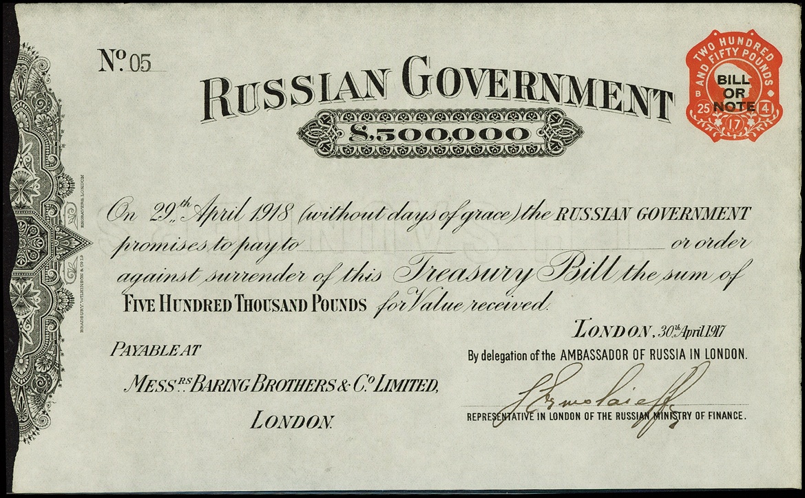
Western markets initially took a hit too, New York Stock Exchange temporarily closing to stop worries about a sell-off. However, after taking a brief hit, most markets in the West quickly recovered. Big investment funds survived, and life soon went back to normal — except for LTCM. They had for example invested heavily in securities that were priced differently across markets. But with the financial downturn, investors turned asymmetrically to securities perceived as "safe", like US treasury bonds, driving the price of LTCM's portfolio further down. Their bet was that these prices would come up again due to the elimination of arbitrage. But it didn't come up in time to save them. You can see the comparison of the LTCM portfolio to the Dow Jones Industrial Average and to US treasury bonds during this period below.

The value of $1000 invested in LTCM compared to $1,000 tracking the Dow Jones Industrial Average, and in U.S. Treasuries at constant maturity.
LTCM lost unimaginable quantities of money, quite literally, during this time. When Russia defaulted they lost $500 million USD in a single day. Their debts were around $100 billion. That's kind of hard to imagine, so let me put it this way: there are 317 million people living in the United States. LTCM debt amounted to over $1,500 for each person in the country. They had made bets amounting to over a trillion, and were doing business with nearly every major firm in the United States and many in Europe. Now, if you're $100 billion dollars in debt, and you're asked to pay back 3% of that, you're being asked to pay $3 billion. If you don't have that kind of money on hand — and at its worst, LTCM did not ‐ then you're done. Worried about a global financial collapse, the US government initiated a massive bailout, and LTCM was ultimately closed.
There were many aspects to how LTCM came to fail. But what is often lost in discussions of LTCM is that several of the assumptions underpinning their models failed too: there was heavy arbitrage in the market, and the risk-free interest rate was not as well-understood as was previously thought.
Failure of random walks: volatility smiles
The Black-Scholes formula is not what ultimately determines the price of an option. Like all financial products, when an option is for sale its price is determined by the buyer and the seller. The Black-Scholes equation simply asserts a prediction about that price given that its assumptions hold.
From its inception, the Black-Scholes formula was incredibly accurate in predicting the price of an option on the open market — that is, accurate until 1987, when for some reason that is not very well-understood, one aspect of it changed.
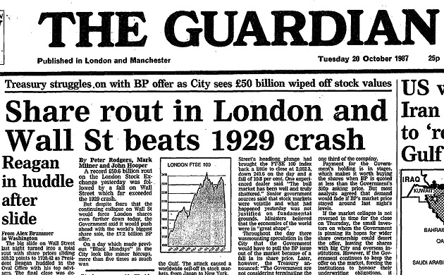
The stock market crash on 19 October 1987 or "Black Monday" was the largest worldwide stock market crashes since 1929. It began in Hong Kong spread arond the globe, plunging markets into historic losses. The Dow Jones Industrial Average lost over 22% of its value. Against the predictions of most economists, the market quickly rebounded, with the Dow Jones returning to its pre-crash closing by 1989. However, option-pricing changed forever, in that the Black-Scholes formula was no longer predicted option prices accurately. The origin of this problem appears to be a systematic failure in the random walk hypothesis.
Recall that, according to the random walk hypothesis, the rate of return of a stock satisfies three conditions: it is equally likely to go up and down, displays roughly equal step sizes, and each step is statistically independent of the previous. This implies that the rates of return are normally distributed, with some fixed variance or "spread", which can be determined by looking at past prices of the stock.
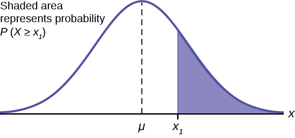
We sometimes refer to that variance as "volatility", since it is a measure of how much a given stock price may swing around.
In deriving the Black-Scholes equation, that variance is used to identify the probabilities associated with future prices of the stock. That is, we think that for the underlying stock we know the variance, and so we use it to predict the option price.
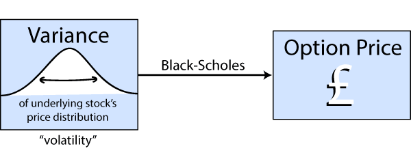
Given that you know the strike price and risk-free rate of return, you can determine the option price given the volatility.
However, it is in principle also possible to work backwards and do the opposite. Suppose we know the option price as it's listed on the market. Then we can use the Black-Scholes formula to predict the variance of the underlying stock distribution. This is just like taking an equation like \(y = 2x + 3,\) that expresses \(y\) in terms of \(x\), and turning it into an equivalent equation \(x = (y-3)/2\) expressing \(x\) in terms of \(y\).
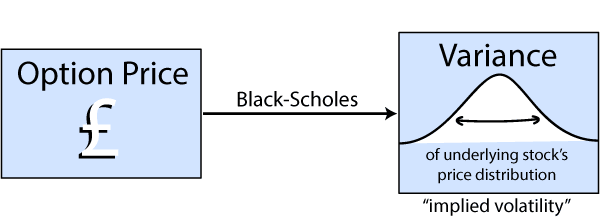
Given that you know the strike price and risk-free rate of return, you can also determine the volatility given the option price.
The variance you calculate when you work backwards in this way is called the implied volatility --- it is "implied" in that, if all the other variables appearing in the Black-Scholes formula are known including option price, then the formula implies a value for the volatility.
This was a useful trick when it was realised that the Black-Scholes formula was no longer predicting the correct option prices after 1987. So, a natural idea was to work backwards and begin with market prices for options, and then work backwards to calculate the implied volatility.
When you do this, what you find is that before 1987, the implied volatility of a stock was completely independent of the strike price of the option. But after 1987, it began to be the case that implied volatility changes with with the strike price of the option, as in the plot below.
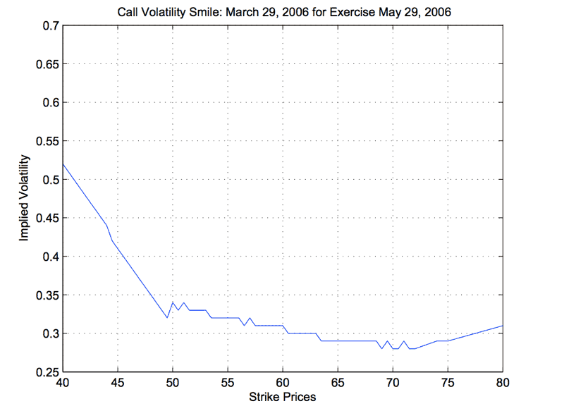
"Volatility smile" in the plot of implied volatility given known crude oil option prices and strike prices
Because of it sometimes resembles a crooked smile, this correlation is called a volatility smile. It suggests that, after the 1987 crash, a low strike price (i.e. an option to purchase for a low price in the future) was viewed as higher volatility and "riskier" than what was suggested by original Black-Scholes equation.
Prior to 1987, and according to the original Black-Scholes equation, the variance of the underlying stock should have absolutely nothing to do with the strike price of an option. A graph like the following would thus be predicted.
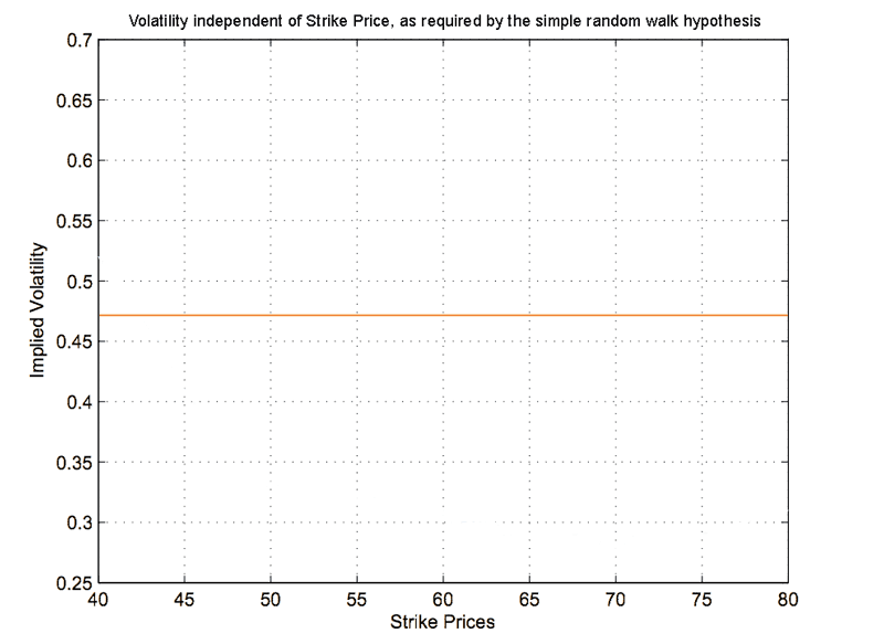
If the underlying stock variance arises from a random walk, its variance should be insensitive to the choice of any given strike price for an option.
Volatility smile is an indication that there are situations in which the random walk hypothesis break down. It turns out this is only the beginning of trouble for the random walk hypothesis.
Beyond Simple Random Walks
Enter Benoit Mandelbrot
The fundamental physicist's thought in random walk theory, which traces its routes to Einstein, is that random walks connect microscopic and macroscopic descriptions. In the case of markets, this means connecting the average behaviour of an individual price to the behaviour of the market as a whole. Can we preserve this thought, even if the random walk hypothesis sometimes fails in finance? We there be a closely related alternative to the ordinary random walk?

Is there an alternative way to get "jiggling" without an ordinary random walk?
The answer turns out to be yes. One of the most important, creative alternatives to the ordinary random walk was developed from one of an eccentric mathematician named Benoit Mandelbrot.
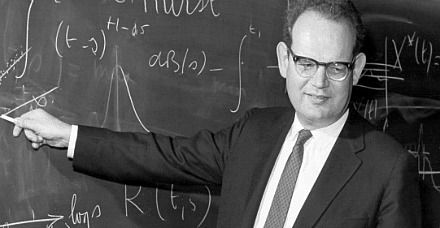
Mandelbrot was a Polish-born mathematician, who moved to France and then the United States, where received a masters degree in aeronautics and then spent most of his career working in a research lab for IBM, finally retiring in 2005. And he had a knack for mathematical peculiarities. For example, he discovered what is now known as the Mandelbrot Set, which displays remarkable scaling structure, as you can see in the following video that continuously zooms quite a long ways into the Mandelbrot set.
We will return to the significance of this sort of structure shortly. Let's look first at Mandelbrot's direct discoveries for finance.
Lévy flights and cotton prices
One of Mandelbrot's central interests in the 1960's, which he reports learning about after picking a paper out of a waste-bin, is the idea that random walks might be replaced with a process in which steps of larger size occur from time to time. That is, instead of a nice, evenly-stepped random walk, Mandelbrot was interested in walks that often involve large, irregular jumps.
Mandelbrot referred to this kind of walk (in which there is a large, irregular distribution of step-sizes) as a Lévy flight after his PhD Paul Lévy, the mathematician who first studied the sorts of distributions that such a walk generates. These distributions have been found to have many useful applications in physics, from the study of turbulence to the distribution of stars in a galaxy.
Mandelbrot had been studying how some of the strange effects described above can arise in probability distributions, when he stumbled onto a chart showing evidence for them in cotton prices. For each 50-day period between 1900 and 1905 (he numbered them approximately 1 through 30), Mandelbrot calculated the `step-size', i.e. the average daily change in rate of return, for cotton in the US commodity market over that period. Since the step-size is roughly the same on the random walk hypothesis, these rates of return should change very little and remain close to the average daily change over the entire 5 year period. But they do not: the step-size varies wildly over the period. One way to account for this would be to say that the variance changes over time. But Mandelbrot immediately recognised it could also indicate that cotton rates of return are described by a Lévy flights.
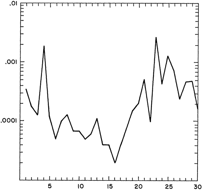
Mandelbrot's (1963) plot of how the 'step-size' (vertical axis) changes over time (horizontal axis) for cotton between 1900 and 1905, with each of the 30 consecutive 'steps' consisting of an average daily change in rate of return over a 50-day period.
Optional: Read the Original Mandelbrot Article
Mandelbrot had discovered that Lévy flights are not mere mathematical curiosities, but may have a basis in empirical economics. Moreover, walk underpinning this distribution was a clear violation of the ordinary random walk hypothesis, and certainly did not give rise to a normal (or 'Gaussian') distribution for rates of return. This led Mandelbrot to write:
"According to... [the random walk] model, these sample means should already have stabilised near the population mean. Since no stabilisation is in fact observed, we see conclusively that the price of cotton did not follow a Gaussian stationary random walk." (Mandelbrot 1963)
The implications of this result are far-reaching. As we have seen, the entire Black-Scholes pricing model depends on the ordinary random walk hypothesis. However, to understand the implications of Lévy flights in the stock market, Mandelbrot needed a more precise way to describe his strange new random walk. In particular, he needed a way of saying what a 'large, irregular jump' is, and how they are distributed. In answering this question, Mandelbrot discovered one of the most famous objects in mathematics, to which we will now turn.
Fractals and fractal dimension
Fractals are often motivated by structures like cauliflower, which has the curious property that if you cut off a piece, it looks remarkably similar to the whole, only smaller.

Cauliflower displays the property of being self-similar.
You might have heard of fractals as being characterised by the property that they are self-similar, in that the whole has a shape that is similar to the part. This is not strictly speaking correct: fractals are not always self-similar, although some of them certainly are. The word 'fractal' refers to 'fractional dimension' in a certain sense that we will now describe.
You are familiar with a certain intuitive definition of dimension: a square is two-dimensional, a cube is three-dimensional, and so on. The dimensions of a few common shapes are illustrated below.
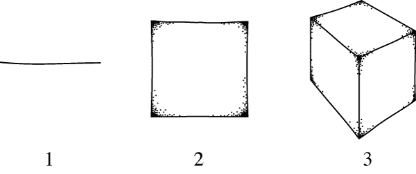
Objects of 1, 2 and 3 dimensions
Here is one more precise way to understand dimension: suppose we measure the size of an object using rulers. How does the measured size change when I split my ruler into 2 pieces? Let's think through a few examples. When I use half a ruler to measure it, the line breaks into 2 pieces. The square breaks into 4 pieces. The cube breaks into 8 pieces. That is, the size of the objects go as follows:
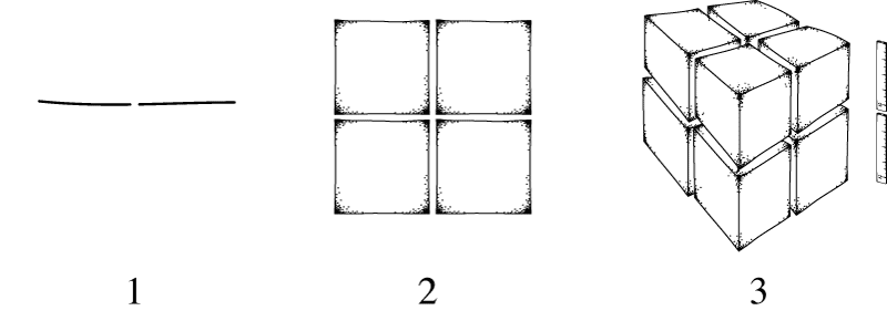
How the size changes when 2 half-sized rulers are used to measure the size of the objects in 1, 2 and 3 dimensions
That is, we find the line's size in the new units is: \(2^1 = 2\). But when I split a ruler that measures the side of a square into two parts, I find that the size of my square goes up to \(2^2 = 4\). The cube size goes up to \(2^3 = 8\). If you think about it for a minute, you'll also see that if I were to split my ruler into 3 pieces, I just get \(3^1 = 3\) for the line, \(3^2 = 9\) for the square, and so on. Thus, we have the following rule: if I split my ruler into \(n\) parts, then I get the relation:
\[(ruler\,parts)^{dimension} = size\]This gives us a neat general rule for determining the dimension of an object. So, according to this rule, what is the dimension of the following shape, called the Sierpinski triangle. To create it, begin with a triangle, delete the central triangle, then delete the centre from the remaining triangles, and so on as shown below.

Creating a Sierpinski triangle by deleting triangles from each central region ad infinitum

If the side-length of the Sierpinski triangle is measured using 2 half-sized rulers, the shape in its entirety triples.
If I split a ruler that measures the side of the triangle into two parts, then it seems that the size of the Sierpinski triangle will triple, since intuitively the whole triangle is just the composition of these three parts. Thus, applying the same rule for determining dimensions I get that
\[ 2^{dimension} = 3. \]What number of dimension does that turn out to be? You can figure this out by taking the logarithm of both sides, from which you learn that the dimension is approximately 1.584. That is, the triangle has fractional dimension. It is for this reason that we call it a "fractal". This may not be an intuitive notion of dimension as you normally imagine it, but it is perfectly well-defined according to the rule above!
Optional: Watch a video introducing fractal dimension
Optional: A precise mathematical definition of fractal dimension
Fractal dimensions can be applied not only to abstract objects like the Sierpinski triangle, but to real-life phenomena like the coastline of Great Britain. The coast is so jagged that we can generally only study its average position using a straight ruler. Moreover, if we use half-sized rulers, we find that the length of the British coastline increases by a factor of about 2.3. So, by this standard, the coastline of Britain has dimension f approximately 1.21.

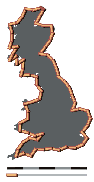
The coastline of Great Britain varies wildly depending on the length of the rulers you use to measure it, giving rise to a fractal dimension.
How does this apply to finance? Mandelbrot realised that, although it is in general hard to describe the "irregular step-size" associated with a Lévy flight, he could make it simple and precise by proposing that the Lévy flight has fractal dimension. Then, the size of the dimension would give an indication of just how "irregular" the random walk is.
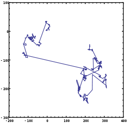
Mandelbrot went on to propose that random walks with fractal dimension would give rise to a distribution, the same way ordinary random walks give rise to a normal distribution. The distribution that they turn out to give rise to is known as a fat tailed distribution. These can be misleading, because they are often very similar in shape to a normal distribution.

But the particular fat tailed distributions that Mandelbrot argued best describe cotton prices have extremely large or even infinite variance. That is, the fatness of the tails is enough to make the average amount that the random walk "spreads out" infinite. Since variance is used in the ordinary Black-Scholes option pricing formula, Mandelbrot's model requires dramatic revision to these models if it is correct.
Mild versus wild randomness
It is a difficult open question as to whether markets are described by fat-tailed distributions and Lévy flights. More generally, it is a difficult open question to determine what the appropriate distribution and appropriate stochastic model for the description of markets. Mandelbroit's models show that they need not merely be "mildly" random, but may be "wildly" random as well (a distinction that Mandelbrot himself introduced).
Mandelbrot's example also illustrates how certain quantities that are often presumed to be empirically measurable are in fact too big to model, or even ill-defined in the classical random-walk framework, such as the variance of the distribution. One must think carefully about the basic terms appearing in Black-Scholes-Merton theory. If we don't input the right information the theory may turn out to give wrong predictions, or even worse, results that are totally meaningless.
You can see Mandelbrot talking about his theory in a TED talk below.
