Overview

In 1971, a new standard of empiricism was introduced into market analysis, as well as an extension of Osborne's treatment of prices in terms of random walks, both familiar ideas inspired by physics. The result is what is known as Black-Scholes-Merton theory. To introduce these ideas, we begin with a discussion of how options can be used to mitigate risk. We then introduce a simple option-pricing strategy that forms the basis for Black-Scholes-Merton theory. This will allow us to illustrate the derivation and significance of the full Black-Scholes equation.

The options paradox

Why love options

Investment is scary. When you do it, you're generally taking something valuable (your hard-earned money) and putting it in an uncertain place. We saw in Lecture 6 how a futures contract can help reduce that risk, by guaranteeing the occurrence of a sale. That is part of the magic of derivatives in general: derivatives can help mitigate risk. Here is one way that this can happen with an option.

Say you own three shares of Facebook stock. You hope the price will go up, in which case you'll make money. But you also worry about the risk that it will go down, and you'll lose money.

You can mitigate some of this risk by sharing it with another person. To do that, you can sell a call option as a kind of 'insurance' against a price drop. Say you sell a call option that gives the owner the right (but not the obligation) to buy one of your Facebook shares for £100 at the end of the year. This promised price for the sale is called the strike price, £100 here. You put the option on the market for a fee of £10, called the option premium. What can happen now? If the price of Facebook goes up, then the buyer will exercise the option and buy your share, since they can make money that way. That's why they bought the opportunity. On the other hand, if the price of Facebook goes down, then at least you made some money from the premium. Selling a call option reduces a little risk at the cost of reducing a little opportunity as well.

The problem of defining risk

There are two competing psychological experiences in the scenario above: the possible reward if the stock price goes up, and the possible penalty if it goes down. Most people are willing to take a little risk. But at some point the risk becomes too much, and you will want a little compensation. When is that point? How much will it be? In other words, how much are you willing to risk on a bet that Facebook's stock price will go up? To decide on an appropriate premium price for the call option you sell, you will need to answer this question.

However, this sort of question sounds suspiciously like a subjective gambling decision. How much are you willing to risk on your poker hand? How much are you willing to risk on Facebook stock? But similar or not, gambling is in many places illegal, whereas investment is not. The general dogma was that every proper financial product must be directly tied to a concrete exchange of goods, as with traditional futures contracts, to distinguish itself from gambling. Thus, options like the one proposed above were forbidden in most financial markets until the 1970's.

Black, Scholes and Merton solve the problem

This policy was changed forever in 1971. In that year, a young applied mathematician named Fischer Black and two economists, Myron Scholes and Robert Merton, made a mathematical discovery that launched a new era of investing. Their simple aim was to derive an objective, empirical means of assigning a price to an option, which depends on market facts rather than individual dispositions. The mathematical theory that made this possible is now known as Black-Scholes-Merton theory.

Black, Scholes and Merton

Simple option pricing

Risk-Free Portfolios

As a first step towards option pricing, let us ask a more general question. In certain table games like Blackjack, it is possible to arrange a tilt the odds in your favour, for example by counting cards. An even better situation would be if you can remove risk from the game altogether, and guarantee yourself free money. Is it possible to do this in the stock market? Something like this is indeed possible; this is known as the concept of a risk-free portfolio.

Recall that in the stock market, it is possible to sell something even if you don't have it. This is called "short selling" or "shorting". Unlike con artists, traders are obligated to deliver on the contracts they sell, and the stock exchange will make sure of it. For example, if you pledge to sell a share of your Facebook stock, and you don't actually have that stock at the end of the year, then you'll just have to go into the open market and buy it in order to ensure delivery.

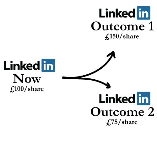
Now, consider a simplified situation in which the price of LinkedIn stock, which is currently £100, can only do one of two things. Suppose that after a year it will either go up to £150, or down to £75. If that is the case, then you can arrange things so that you are guaranteed to make £50, without any risk at all. All you have to do is short sell in the following way.

Instead of buying an entire share of LinkedIn, suppose you buy 2/3 of a share. You then write a call option for someone to purchase an entire share of LinkedIn from you for £100, with the transaction place to take place in one year, even though you doesn't actually have that much LinkedIn stock.

The possible outcomes for the stock and for the call option are given below.

Outcome 1: Stock goes up. If the stock goes up to £150, then the option-holder will exercise her option to buy a LinkedIn share at a cheaper price. So, she'll give you £100, and you'll have to give her a share in return. You don't have a complete share, only 2/3 of one, so you'll have to go buy the remaining 1/3 at market price of £150 × (1/3) = £50 and give it all to the option-holder.

Your Net Gain: £100 - £50 = £50.

Outcome 2: Stock goes down. If the stock goes down to £75, then the option-holder will not exercise her option, since she can buy LinkedIn shares cheaper elsewhere. So, you'll simply keep your 2/3 share of LinkedIn, which is now worth £75 × (2/3) = £50.

Your Net Gain: £50.

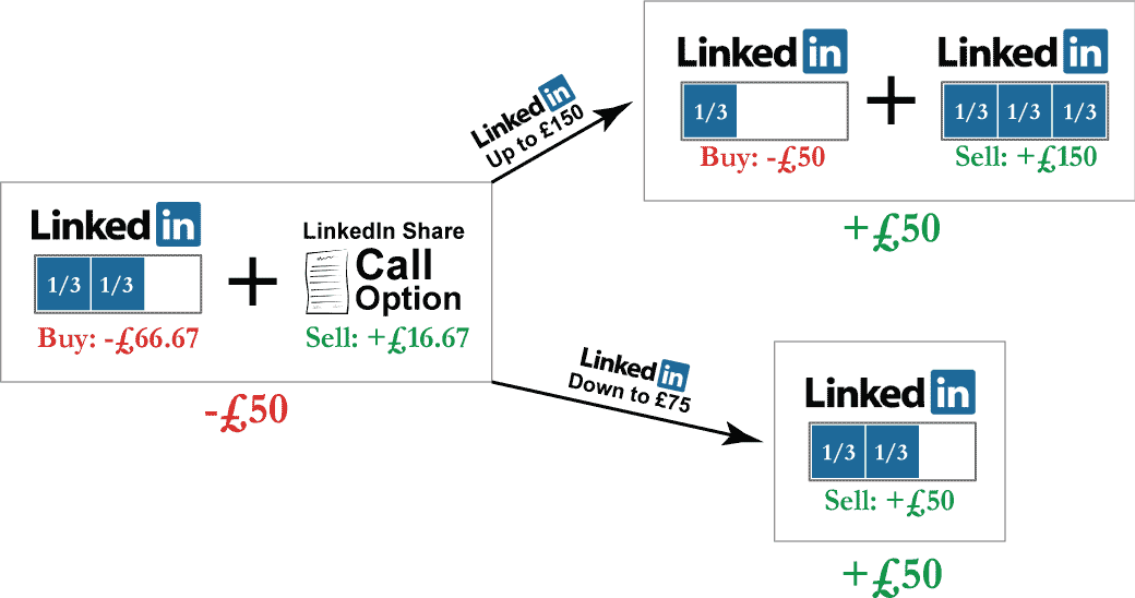
Risk-free portfolio (assuming a 0% interest rate)

The result is the same either way: you earn £50, risk-free, with certainty. Of course, you already spent £66.67 in order to acquire your 2/3 share of LinkedIn stock. You actually begin this scenario in the hole by -£66.67. So, what would be a fair price for you to charge for your call option? It would be £66.67 - £50 = £16.67, so that you break even (assuming, for the moment, that there is no interest). Only then would the buyer of the call option agree that you're not charging too much.

This suggests that, at least in this special scenario, there is a definite, fair price for a call option, which has nothing to do with anyone's special psychological attitude toward risk.

Risk-Free Interest and the time-value of money

There is a further subtlety about the risk-free portfolio above. The way we have described it, you invest £50 now, and receive £50 later. But in the meantime, you must live without your £50! That participants in a market expect to be compensated for being without their money is called the time value of money. Indeed, it is exactly this situation that gives rise to the interest rate that you receive in your bank savings account, as we discussed last time.

This means that, in the example above, you should actually arrange things so that your costs are less than £50, but in such a way that that they grow with interest to be worth exactly £50 on the exercise date. How do we do that? We must first discount your future earnings given the interest rate to find out whatever that "future £50" is worth today. We should then set the premium price of the call option so that your total costs are equal to this discounted value. If the interest rate is 10%, then then your future £50 is worth about £45.45 today, and so the Call Option premium should be £21.22.

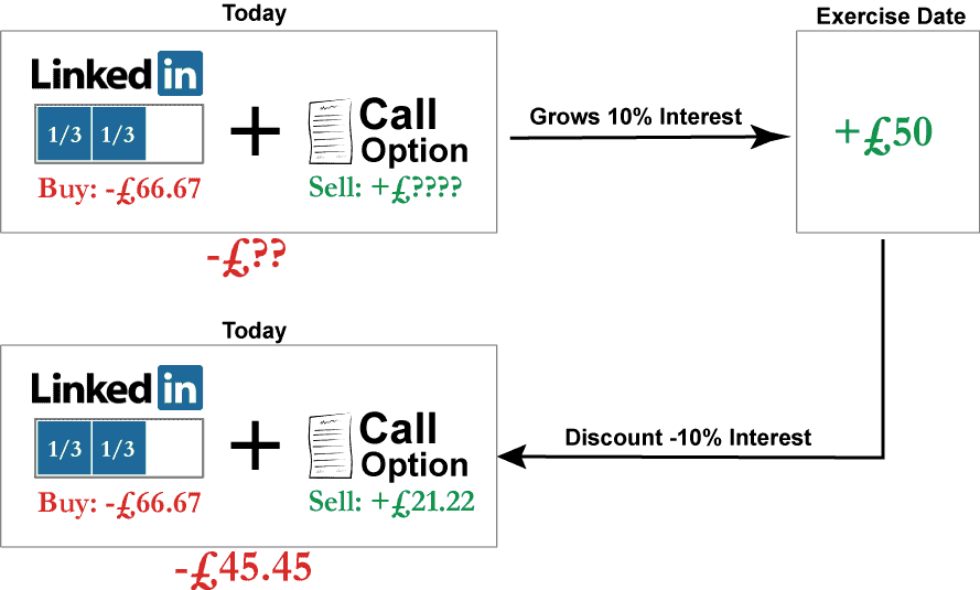
Discounting future earnings to learn the corresponding price today and determine an appropriate Call Option premium.

The portfolio we have assembled, of 2/3 a share of LinkedIn plus the sale of a call option, has the remarkable property of being "risk free". There is no uncertainty about the future (assuming as we have that there are only these two possible outcomes.) We are guaranteed to receive £50 on the exercised date. So, this scenario is like a highly desirable loan, in which there is a 100% guarantee that you will get your money back.

How can we determine the interest rate for such a scenario? We would need to find a comparable scenario, perhaps at a lender with an incredibly reliable means of generating revenue, providing an effective guarantee that money on a loan would be paid back. Whatever interest rate such an institution would use for its loans could be used to measure interest rate in the absence of risk, and thus provide an appropriate interest for our risk-free portfolio above. So, does such an institution exist?

Stable governments can pay back their loans very reliably due to their ability to raise tax revenue.

Sure it does. For example, the UK and US governments take out loans in the form of government bonds. The potential of these institutions to pay back loans is extremely reliable, as they are always able to raise revenue through taxes, and even print money if they need to. Indeed, economists once thought that it would be impossible for a developed country to default on its loans. This proved to be strictly incorrect when in 1998 the Russian Central bank defaulted on its debt, as we will discuss next time.

Government bonds thus provide one reliable means of empirically measuring an appropriate risk-free rate of return. US investors often uses the rate of return on a 3-month US Treasury bill. On 27 February, 2017, that rate of return was 0.51%.

Options for all portfolios: no-arbitrage

We have developed a fair way to price an option in our special risk-free portfolio. But what if someone were to sell an arbitrary option for LinkedIn shares? Should the price of the Call Option premium change if we happen to have a different portfolio that doesn't guarantee a fixed rate of return? In many contexts, it makes sense to assume that the answer is no: a given Call Option premium should cost the same in all contexts.

One common argument for this is from the impossibility of arbitrage among investors sharing publicly available information. This begins with the hypothesis that markets in general display a high degree of efficiency in the sense that one cannot guarantee a profit by purchasing something at a lower price in one place and then selling higher in another. Such a guaranteed-profit mechanism is called "arbitrage", as illustrated with bananas below. It is often said to be impossible in general public markets, and there is some empirical evidence to support this under certain circumstances.

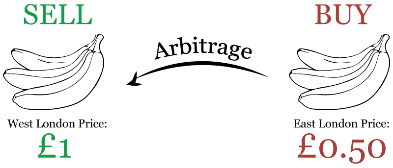
The idea is that, if an arbitrage opportunity were to arise, it would disappear very quickly. For example, if East London banana sales are going for cheaper than West London sales, then increased demand arises as people make a guaranteed profit buying from one and selling to the other. This drives the price of East London bananas up. In the case of the stock market, arbitrage opportunities are typically recognised by corporate leaders and employees long before they make it into the public. As a result, by the time the price has adjusted on the public market, all possibilities for arbitrage typically disappear.

The same goes for the LinkedIn call option we have described above. You might not have a risk-free portfolio when you choose to sell that option. But the point is, you could build a risk-free portfolio if you wanted to, and it would have the fixed price indicated above. If anyone ever sold that Call Option for more or less than the risk-free premium, then we could make a risk-free profit by purchasing at the lower price and selling at the higher.

Such arbitrage opportunities are not impossible, and money can be made when they are discovered. However, in general open markets with good information flow between a large number of participants, arbitrage is extraordinarily rare. When this is the case, the risk-free premium is also the general premium when purchasing an option.

Here then is a summary of our simple option pricing strategy.

Simple Black-Scholes style option pricing summary

The Black-Scholes Equation

The most unrealistic feature of the simple pricing strategy above is that it dramatically simplifies future possibility, through the idealisation of only two future outcomes. But apart from that, our simple strategy is not so complicated, and exceedingly clever. It is something you might even have thought of in the shower, on a good day.

The Black-Scholes pricing follows the same strategy, but just removes the idealisations. The equations expressing this fact appear complicated at first, but the philosophy underpinning them is actually quite simple, and closely related to the physicists approach to modelling. Here is how they work.

A physicist's approach to pricing

Fischer Black began his career as a physics undergraduate at Harvard. In graduate school he decided to switch from mathematical physics to pure mathematics, then to artificial intelligence, and then was finally kicked out of School for failing to complete his courses. So, he began working for a financial consulting firm instead. (Harvard later awarded him a PhD for his research anyway.)

From a mathematical physicist's perspective, the pricing strategy above is an incredible, dramatic improvement in our understanding of options because it deals with entirely measurable quantities. We don't need to know anything about an amorphous concept of "individual risk aversion". We can empirically measure the risk-free rate of return, and that's enough. Similarly, we might need to know the possible future outcomes associated with a stock price, or more generally the distribution of rates of returns. But that too can be measured empirically on the basis of past rates of returns. The simple pricing strategy above is important because it reduces the problem to measurable quantities. This is one of the characteristic strategies of theorising in physics as well, as in Galileo's description of free-fall in terms of only a body's height above the ground.

In the simple option pricing strategy above, the quantities we needed in order to determine the price of an option were only the following.

Empirically measurable quantities for Black-Scholes pricing

This final item, the distribution of rates of return, is the piece of information that tells us what the underlying stock price might be in the future. In our simple model, there were only two possibilities, £150 or £75. In general, there is everything in between and more.

So, to generalise our simple pricing strategy, we just need a way of filling in all those other possibilities. To do that, we turn to the random rate of return hypothesis and the resulting normal distribution on rates of return.

Random walks and probability

Recall from last time that if a stock price is written \(P = e^{rt}\), then \(r\) is called the rate of return. As we saw, there is reason to think that in many markets, the rates of return can be modelled as following a random walk, and therefore are will be normally distributed with some variance, which we assume is fixed. This occurs when there are huge numbers of market participants that are relatively uniformly spread around all the possible buying and selling positions.

Normal distributions have the very convenient property that the probability of an occurrence at or above some value is equal to the area under the curve after that value.

Probability associated with a normal distribution.

So, as long as we know the we have a fixed-variance normal distribution we can easily calculate the probability that a rate of return will go above a certain value. Why is that interesting? Because we can use it to calculate the probability that the stock price will go above the strike price of an option, in which case we would expect the option to be exercised; that is, this corresponds to the case that "the price goes up" in our simple option pricing model above. Here is how we can put this fact to work.

The full Black-Scholes solution

Our simple pricing model is known as a binomial model for option pricing. As we let the number of possible future increase to infinity, we find that we need a way to control how likely each outcome is. For this, we use the distribution of rates of return above. This gives rise to a formula for the price of an option known as a Black-Scholes solution. It was first written down by Fischer Black and Myron Scholes in 1971. It expresses the price of an option in terms of the current price of the underlying stock, the variance associated with the normally distributed rates of return for stock, and the risk-free interest rate associated with a some government bond. The Black-Scholes solution then takes the following form.

Black-Scholes Solution: \(P = (F - K\times p)\times e^{-RT}\)

Optional: More formal details

• \(P\) is the price of the option premium, given that it expires at time \(T\) in the future. This is what we want to calculate.bl
• \(F\) is the expected future value of the underlying stock price conditional on the case where the stock price is excercised; i.e. given that the future price of the stock at the time \(T\) of expiration is greater than the strike price \(K\).
• \(K\times p\) is the strike price weighted by the probability \(p\) that the option is exercised, i.e. that the future price of the stock at the time \(T\) of expiration is greater than the strike price \(K\).
• \(e^{-RT}\) is a factor that discounts the resulting future value of the option price to present-day terms, by a rate \(R\) that is the risk-free interest rate associated with a government bond.

In sum, the Black-Scholes formula says that an option is equal to the future value of the stock (given that the option is exercised) minus the expected strike price (given that it is exercised), all discounted to present-day terms using the risk-free interest rate. This is the full "continuous analogue" of the simple binomial model discussed above.

In practice we normally begin knowing a fixed initial stock price \(S\) and a strike price \(K\). The probabilities in the Black-Scholes formula can all be determined using the variance of the normal distribution for the stock's rates of return, and everything else (such as the discount rate) can be determined using the risk-free rate of return. So, the option premium price \(P\) is actually only a function of the variance \(\sigma^2\), sometimes called the "volatility", and the risk-free interest rate \(R\).

All of this works because of the assumption that the underlying stock follows a random walk. Thus, the formulation of the Black-Scholes equation was ultimately made possible by modelling trade events as being like a giant swarm of water molecules, just like the models developed by Einstein.

As a diffusion equation

What is commonly called the Black-Scholes equation is a differential equation that expresses how the option premium in the Black-Scholes solution changes given different expiration times. This equation says that the rate of change of the option premium as you increase the expiration time is proportional to the so-called concavity with respect to the underlying rate of return. This can be understood visually by imagining the option premium is analogous to heat on a pipe, and the different positions on the wire correspond to different temperatures.

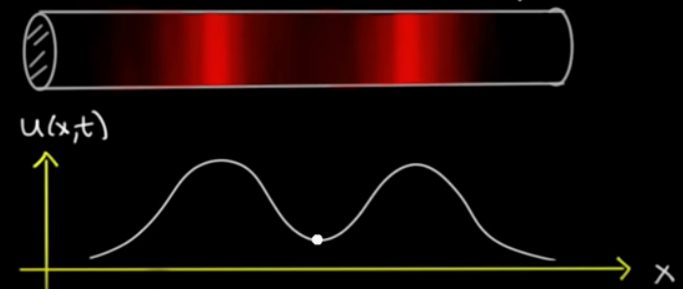
Think of the different positions on the pipe as corresponding to different rates of return, and the function \(u(x,t)\) is describing the price of the premium. Then, like heat on a pipe, the Black-Scholes equation says that the rate of change of the premium price with respect to the expiration time will be faster where there is more "concavity" (or a "sharper curve") on this graph. In physics, this leads heat to spread around the pipe until it is in equilibrium. With option pricing, option premium tends to spread more evenly across the rates of return.

If you are interested in the technical details of the heat equation, try this video (optional).

Further spreading of risk

Risky investments can of course lead to some very big payoffs. But not everybody wants to take on that risk. How else can you avoid it?

One way is to avoid risk is to have a wide-ranging, diverse collection of stocks. Many of the risks of loss in a stock are tied to special facts about that company. For example, there might be a risk that some company headquarters will get hit by a hurricane, or that its CEO will alienate all the employees and leads them all to quit. Either of those things could cause the stock price be different from what you expect. But that kind of risk can be avoided just by purchasing many different stocks. That way, any the potential loss from one investment will typically be offset by gains from another.

However, not all risk can be diversified away. The stock market average itself goes through dramatic upward and downward swings. And all stocks tend to swing up and down with the average, although some do more than others. This deviation from the expected price is often called "systematic risk" because it is thought to be a risk inherent in the market. It is not due any special facts about a company.

The S&P 500 (left) is one measure of the average behaviour of the American stock market. Some of the changes in stock price for an American company like Ford Motor Company (right), such as the big dip during the 2008 crash, are correlated with the S&P price.

Thus, it is often desirable to mitigate risk using other means, and for this purposes options can be very useful if their price can be understood in a controlled way. After the discovery of the empirically based, randomly walking Black-Scholes pricing model, this possibility seemed more optimistic than ever.